2.2. Semantic Search

Semantic search is a technique that, instead of searching for specific words, aims to search for the contextual meaning of those words. Unlike lexical search, which only searches for literal matches of words, semantic search tries to understand the user’s intention and the overall sentence’s meaning.

2.2.1. Word and Sentence Embeddings

Word Embedding is a mathematical technique and implementation of the Distributional Hypothesis (DH). DH defends that if words appear in similar contexts, they must have similar meanings. Word embeddings provide a verification of which words are similar to each other based on an initial corpus of sentences. Each word embedding represents a word in a multidimensional space. With multiple multidimensional word representations, verifying which words are related to each is possible based on the distance between words.

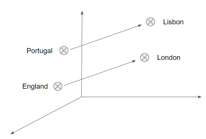
The distance can be calculated through the Cosine Similarity:

\[\begin{split} CosSim(A,B) = cos(\theta) \\ = \frac{A \cdot B}{||A|| ||B||} \\ = \frac{ \sum_{i=1}^{n} A_i \cdot B_i}{\sqrt{\sum_{i=1}^{n} A_i^2} \cdot \sqrt{\sum_{i=1}^{n} B_i^2}} \end{split}\]

Since word vectors are linear systems, it is possible to perform arithmetic operations in the embedding space. If we get a word “England” and subtract the word “London” and add the word “Portugal”, we should be able to get the word “Lisbon”.

\[ Word("England")-Word("London")+Word("Portugal")=Word("Lisbon") \]

There are different implementations of word embeddings, such as Word2Vec proposed by a Google Team in 2013 led by Tomas Mikolov [MCCD13] or Global Vectors for Word Representation (GloVe) [PSM14] developed at Stanford in 2014. Both make use of neural networks to create their models through unsupervised training. Both implementations have their unique advantages, but what distinguishes them mainly are their fundamentals of the solution formulation.

2.2.2. Word2Vec

Word2Vec is a two-layer neural network proposed in 2013 by Tomas Mikolov et al. and it revolves around the idea that words that appear close to one another have similar meanings.

Word2Vec algorithm uses one of two methods that utilise neural networks [Ron16]:

• Continuous Bag of Words (CBOW)

• Skip-gram

CBOW model, through the representation of context using the surrounding words as an input, aims to predict the corresponding word. Considering the example: “I walked through the public garden.”, we can input the phrase without the word “public” in the Neural Network. By using this single input, it aims to predict the word “public” just by interpreting its surroundings.

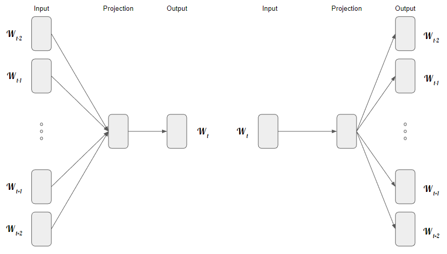
Figure retrieved based on [MCCD13]

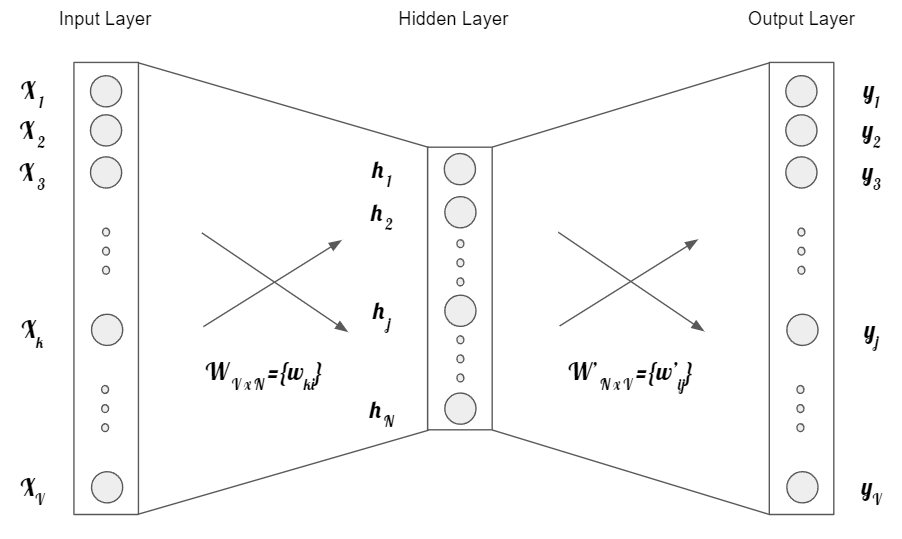
Figure retrieved base on [Ron16]

The input layer, which is the one word that will serve as context, is a vector of size \(\text{V} = \{x_1, ... , x_V \}\). The hidden layer is composed by N neurons, and the output layer is a vector of size V that represents the predicted word. The weight matrix \(W\) has size \( V \times N \).

If the objective is to use multiple words for the context to predict a word, the neural network would need to increase the input layer,

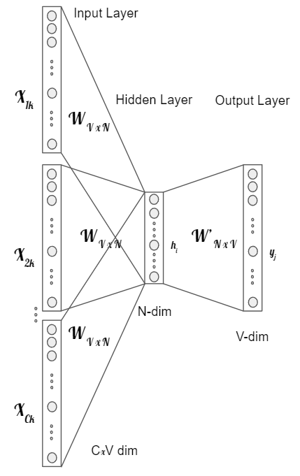
Figure retrieved based on [Ron16]

The Skip-Gram model’s function is to use a word as an input and generate the context of that same word.

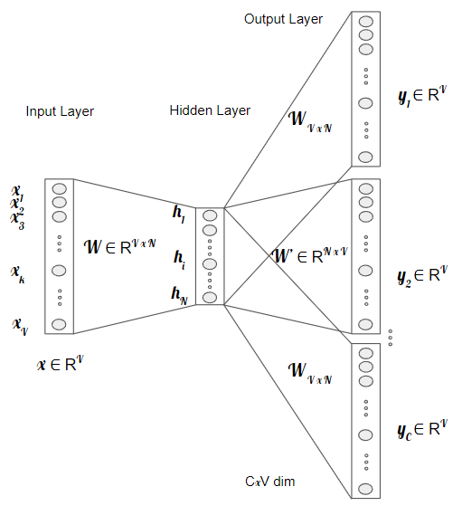
Figure retrieved based on [Ron16]

Word2Vec relies on local information, meaning words are only affected by words in the surroundings. The technique can not associate a word as a stop-word or a word that has meaning in a phrase. Stop words are everyday words that have no complex meaning. For instance, in the sentence: “The cat sat on the mat”, Word2Vec cannot identify if the word “The” is a particular context of the words “cat” and “mat” or if it is just a stop-word. Nevertheless, this technique performs very well in analogy tasks.

• How to use word2vec in python: https://www.geeksforgeeks.org/python-word-embedding-using-word2vec/

2.2.3. GloVe

GloVe is an unsupervised learning algorithm developed by researchers at Stanford University that aims to represent words in vectors. It focuses on the idea that it is possible to derive semantic relationships between words based on a co-occurrence matrix. Each value in the co-occurrence matrix represents a pair of words occurring together.

The original paper demonstrated the co-occurrence matrix produced with probabilities for targets word ice and steam.

The word ice co-occurs more frequently with the word solid than it does with the word gas, whereas steam behaviours in the opposite way. Also, both are related to water* and do not show a strong co-occurrence with the word fashion. The last row shows whether a word relates more with ice (values much bigger than 1), steam (values much lesser than 1) or present a neutral co-occurrence (close to 1).

Co-occurrence probabilities for target words ice and steam showed in the original paper

In a sense, GloVe receives as an input a corpus of text and transforms each word in that corpus into a position in a high-dimensional space based purely on statistics through a co-occurrence matrix. With the produced vectors, it is possible to retrieve related words based on the distance between vectors.

2.2.4. Recurrent Neural Network

Recurrent Neural Network (RNN) is a type of neural network used for processing sequential or time series data, where the input has some defined order. One way to visualize RNN is by viewing the architecture as multiple feed-forward neural networks that feed information from one network to another.

In practice, it is one network where the cells iterate over themselves for every input they acquire

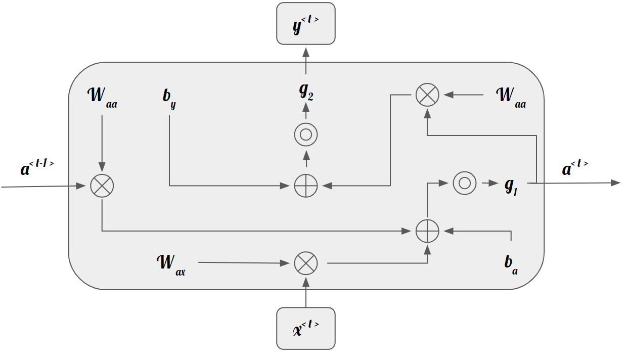
Figure based on https://stanford.edu/~shervine/teaching/cs-230/cheatsheet-recurrent-neural-networks

RNN makes use of a hidden vector that has information from the last iteration. In doing so, its actual vector, \(a^{<t>}\), depends on the previous vector, \(a^{<t-1>}\), and the current input, \(x^{<t>}\). It is defined by the following:

\[\begin{split} a^{<t>} = g_1(a^{<t-1>}, x^{<t>}) \\ = f(W_{aa} \cdot a^{<t-1>} + W_{ax} \cdot x^{<t>} + b_a) \end{split}\]

where \(W_{ah}\) and \(W_{ax}\) represent the weight matrix for the hidden vectors and inputs, respectively, and \(b\) represents the associated bias. Usually, the activation functions used for this \ac{RNN} are either the logistic function (Sigmoid), Hyperbolic Tangent (Tanh), or Rectified Linear Unit (ReLU).

The output vector (prediction), \(y^{<t>}\), depends on the hidden state vector, \(a^{<t>}\).

\[ y^{<t>} = g_2(W_{ya} \cdot a^{<t>} + b_y) \]

where g is another activation function, normally softmax.

This kind of architecture allows the networks to analyse any input with unspecified length while maintaining the model size, taking into consideration historical information, with weights being shared across time.

The loss function used in this architecture has to be defined at each timestep:

\[ L(\hat{y},y)=\sum_{t=1}^T L(\hat{y}_t,y_t) \]

In the training process, the RNN makes use of a gradient-based technique named Backpropagation Through Time, calculated at each point in time. At a timestep, \(T\), the derivative of the loss function, \(L\), with respect to the weight matrix \(W\) is as follows:

\[ \frac{\partial L ^{(T)}}{\partial W} = \sum_{t=1}^T \frac{\partial L ^{(t)}}{\partial W} \]

In the Backpropagation Through Time mechanism, since it is hard to capture long-term dependencies because of the multiplicative gradient, the propagated errors might either tend to zero or increase exponentially (vanishing or exploding gradient phenomena). One method to help deal with the exploding gradient phenomena is by capping the maximum value for the gradient: Gradient clipping. On the other hand, to deal with the vanishing gradient phenomena, several types of gates that have very well-defined purposes are used.

One problem raised by RNN is related to long-term dependencies. Taking into consideration the example: “I like flowers a lot. Today, I walked through the public garden.”. The information that the user likes flowers, should be an indication that he might walk through the “garden”. There is a chance that the distance between the information and the place where it is needed is too large. In these circumstances, RNNs are unable to learn to connect the information. Long Short-Term Memory (LSTM) solve this problem.

2.2.5. Long Short-Term Memory

LSTM network is a variant of RNN that is able to deal with long-term dependencies.

Standard RNNs have a very simple structure, having, for instance, a single tanh layer.

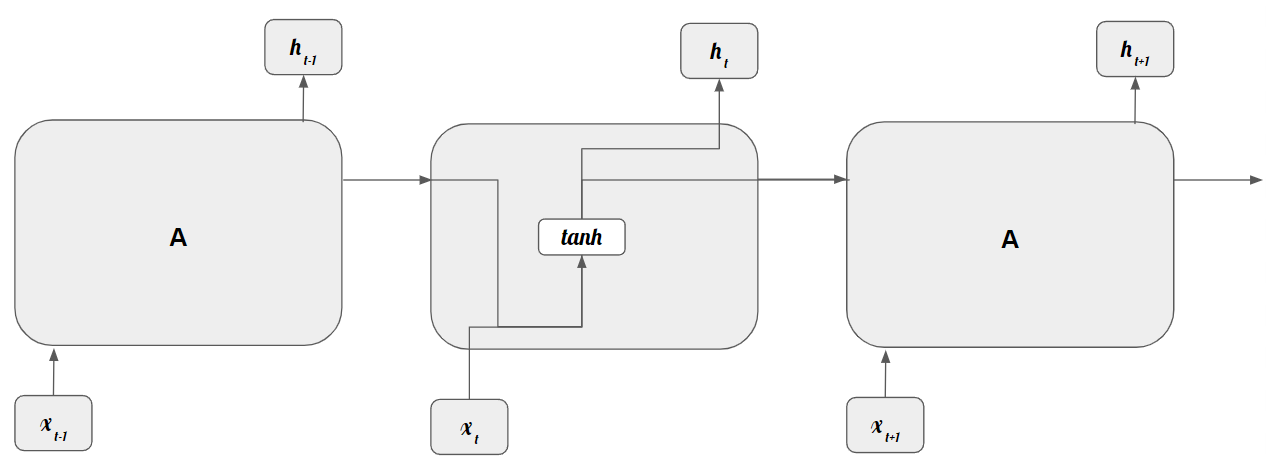
Figure based on https://colah.github.io/posts/2015-08-Understanding-LSTMs/

LSTMs contain a slightly more complex structure. They are specifically designed to tackle the problem with long-dependencies that ordinary RNNs would struggle with.

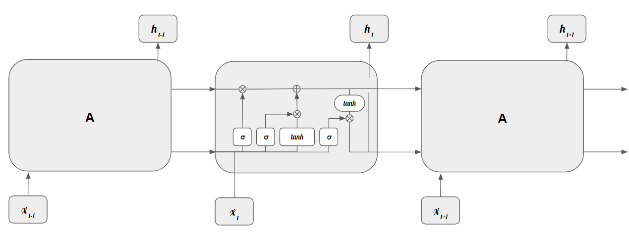
Figure based on https://colah.github.io/posts/2015-08-Understanding-LSTMs/

The cell state, \(c\), flows across the entire chain, interacting linearly occasionally. If the information provided by the cell state is barely changed, it is easy to preserve the information over time. The gates have the ability to remove or add information to the cell state. In Fig. LSTM these gates are represented by \(\sigma\), since they make use of sigmoid functions.

There are three main types of gates: Forget Gate, Input Gate, and Output gate.

The Forget Gate layer is responsible to select which information is staying or not in the cell state. It makes use of a sigmoid function and, by looking at \(h_{t-1}\) and \(x_t\), it outputs a number between 0 and 1 that represents how much information is kept:

\[ f_t = \sigma(W_f \cdot |h_{t-1}, x_t| + b_f) \]

The Input Gate layer aims to determine which values are going to be updated. In conjunction with a tanh layer, it helps determine what information is going to be stored in the cell state.

The Input Gate output is as follows:

\[ i_t = \sigma(W_i \cdot |h_{t-1}, x_t| + b_i) \]

while the output of the tanh layer, the new cell state candidate vector, \(\tilde{C}_{t}\), is given by:

\[ \tilde{C}_{t} = tanh(W_C \cdot |h_{t-1}, x_t| + b_C) \]

This way, the cell state, \(C_t\) is defined as:

\[ C_t = f_t * C_{t-1} +i_t * \tilde{C}_{t} \]

The Output Gate layer is responsible to decide what is going to be, in fact, outputted and, in conjunction with a tanh layer, deciding what is going to be passed to the next cell. The Output Gate is defined by:

\[ \sigma_t = (W_o \cdot |h_{t-1}, x_t| + b_o) \]

This output vector originating from the Output Gate is used to determine the hidden vector, \(h_t\), that is going to be transmitted to the next cell.

\[ h_t = \sigma_t \cdot tanh(C_t) \]

2.2.6. Transformers

Since it is possible to assume that RNNs are unrolled networks that are arbitrarily deep, they might take too long to train (LSTMs even more due to their complexity). Nevertheless, LSTMs, even though they are able to tackle long-term dependencies, due to long training times and the fact that the recurrence prevents the use of parallel computation (widely use in moderns computer processors), a Google Team has suggested a new Neural Network (NN) structure: Transformers. [VSP+17]

Transformers facilitate long-range dependencies, eliminate the Gradient Vanishing and Explosion phenomena, and, by making use of techniques that do not involve recurrence, facilitate parallel computation, reducing the training time.

The encoder is responsible for receiving an input sequence, \begin{math} x = (x_1, …, x_n) \end{math}, and map it into a contextualized encoding sequence, \( z = (z_1, ..., z_n) \). The encoder is composed of \(N = 6\) identical layers where each layer contains two sub-layers, a Multi-Head Attention Layer and a Feed-Forward Neural Network, that produces outputs with \(\text{model} = 512\) dimensions.

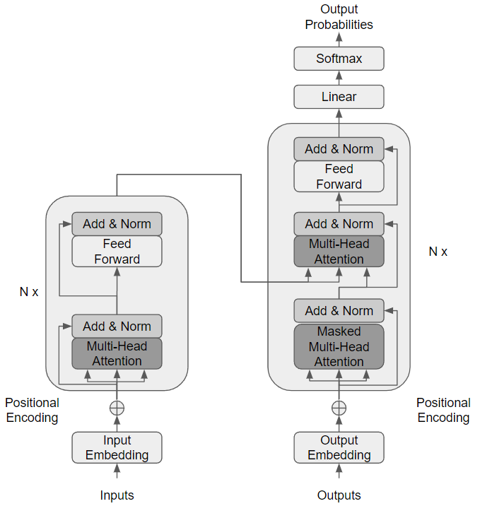
Figure retrieved based on [VSP+17]

The Transformer Model is composed of different components. The Input Embedding is responsible to transform the inputs into a scalar vector and map them into space where words with similar meanings are close to one another. These words might have different meanings depending on their context and position in a sentence. Positional Encoding tackles this problem.

Positional Encoding is a vector that provides context depending on the position of a certain word in a sentence. In the original paper, it is used sine and cosine functions with different frequencies.

\[ \text{PE}_{(pos,2i)} =\text{sin}(pos/10000^{2i/d_{\text{model}}}) \]

\[ \text{PE}_{(pos,2i+1)} = \text{cos}(pos/10000^{2i/d_{\text{model}}}) \]

where \(pos\) is the position and \(i\) is the positional encoding dimension.

After the input is passed through the Input Embedding and the Positional Embedding, it is passed towards the Encoding Block. Here, the Transformer Model contains the Multi-Head Attention Layer and Feed-Forward Neural Network, as mentioned before.

The Multi-Head Attention Layer uses an attention mechanism to assign different weights that, for every word, generates a vector that captures the importance between words of a specific sentence.

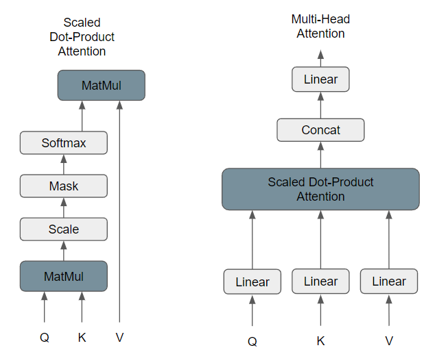
Figure based on [VSP+17]

The attention function receives a query, a key, and a value and aims to pair it to an output. All the inputs are vectors and the output is calculated based on a weighted sum of the values.

\[ Attention(Q, K, V) = softmax(\frac{Q \cdot K^T}{\sqrt{d_K}}) \cdot V \]

where \(Q\) is a set of queries, \(K\) is a matrix with the keys of the words from the query and \(V\) is a matrix that holds the values of the words from the query. The input consists of queries and keys of dimension \(dk\), and values of dimension \(dv\). Instead of running the attention function one time for each set of keys, values, and queries, the original paper states a solution based on projecting linearly the same sets \(h\) times with different, \(dk\), \(dk\), and \(dv\) dimensions, respectively. This way, the projected images of the keys, values, and queries are run in parallel.

\[ MultiHead(Q, K, V) = Concat(head_1, . . ., head_h) W^0 \]

where

\[ head_i = Attention(Q W_i^Q, K W_i^K, V W_i^V) \]

and where the projection matrices \(W_i^Q \in \mathbf{R}^{d_{model} d_k}\), \(W_i^K \in \mathbf{R}^{d_{model} d_k}\), \(W_i^V \in \mathbf{R}^{d_{model} d_V}\) and \(W_i^O \in \mathbf{R}^{h d_V d_{model} }\) and \(h = 8\) parallel attention layers.

Finally, there is the Decoder Block. The Decoder is composed of a Masked Multi-Head Attention layer, a Multi-Head Attention layer, and a Feed Forward layer. Both the Multi-Head and the Feed Forward components are similar to the Encoder Block. When it comes to the Masked Multi-Head Attention Component, there are some differences. This component aims to reduce the bias that might exist toward some words by turning the words that appear after into 0, so they do not affect the calculations.